Column-Level Statistics

Column-Level Statistics are metadata measurements computed over the values in individual columns of data files, stored alongside the data to enable two distinct categories of query optimization: data skipping (eliminating irrelevant files and row groups before reading any data) and cost-based query planning (making intelligent decisions about join ordering, join strategy, and resource allocation based on data cardinality and distribution).

The distinction between these two optimization categories is important and often conflated. Data skipping statistics (min, max, null count) are used at query execution time by the query engine’s scan operators to prune irrelevant storage units. Cost-based optimization statistics (distinct value counts, value distributions, histograms) are used at query planning time by the query planner’s optimizer to select the most efficient execution plan — entirely before a single byte of data is read.

Understanding both categories of column-level statistics, their storage formats, their collection overhead, and their practical impact on query performance is essential for data engineers building high-performance lakehouse environments.

Category 1: Data Skipping Statistics

Data skipping statistics were covered in depth in the Min-Max Statistics article. This section provides a consolidated reference and extends the analysis to additional statistical dimensions.

Min/Max Bounds

The minimum and maximum values of a column within a storage unit (Parquet row group, Iceberg data file). Used to evaluate range predicates (=, >, <, BETWEEN) and eliminate storage units whose entire value range falls outside the query’s filter.

Stored in: Parquet row group footer (per column chunk), Iceberg Manifest File entries (lower_bounds, upper_bounds).

Effectiveness: Maximized when data is sorted or clustered by the predicate column, producing narrow, non-overlapping min-max ranges across files. Minimized for high-cardinality equality predicates on unsorted data, where every file’s range includes the target value.

Null Counts

The count of null values in a column within a storage unit. Used to evaluate IS NULL and IS NOT NULL predicates.

Stored in: Parquet row group footer (null_count per column chunk), Iceberg Manifest File entries (null_value_counts).

A storage unit where null_count = 0 can be skipped for WHERE column IS NULL predicates (no nulls exist). A storage unit where null_count = row_count can be skipped for WHERE column IS NOT NULL predicates (all values are null).

Value Counts

The total number of non-null values in a column within a storage unit (equivalently, row_count - null_count for a non-nested column). Used by query planners for cardinality estimation at the file level.

Stored in: Iceberg Manifest File entries (value_counts).

NaN Counts

For floating-point columns (FLOAT, DOUBLE), NaN (Not-a-Number) values are distinct from null values and cannot be compared using standard comparison operators. Iceberg tracks NaN counts separately to allow query engines to correctly handle floating-point predicates.

Stored in: Iceberg Manifest File entries (nan_value_counts).

Category 2: Cost-Based Optimization Statistics

Cost-Based Optimization (CBO) is the branch of query planning that selects among multiple valid execution plan alternatives by estimating the computational cost of each alternative and choosing the cheapest. The quality of CBO decisions depends entirely on the accuracy of the cost model’s inputs — specifically, estimates of how many rows each operator in the plan will produce.

Without accurate cardinality estimates, the query optimizer must fall back to heuristics and fixed assumptions that are frequently wrong in practice. Common failures include:

• Wrong join order: Joining a 1-billion-row fact table against a 10-row dimension table in the wrong order (using the large table as the probe side instead of the build side) can be 1,000x slower than the optimal order.
• Wrong join strategy: Choosing a hash join when a broadcast join would be 100x faster (because one side is small enough to fit in memory).
• Overestimated memory allocation: Allocating 8GB for a hash aggregation’s hash table when the actual data requires only 50MB, wasting memory headroom and causing unnecessary spills when another query runs simultaneously.

All of these failures stem from inaccurate cardinality estimates. Column-level statistics — specifically distinct value counts, histograms, and value distribution profiles — are the inputs that enable accurate cardinality estimation.

NDV: Number of Distinct Values

The Number of Distinct Values (NDV) for a column is the count of unique values that appear across all rows in the column (across the entire table, not just a single file). NDV is the most important single statistic for cardinality estimation in JOIN and GROUP BY operations.

For a query:

SELECT region, count(*) 
FROM orders 
GROUP BY region

The optimizer needs to know: how many distinct regions are there? If NDV(region) = 50, the GROUP BY will produce 50 output rows, and the hash table needs to accommodate 50 distinct keys. If NDV(region) = 5,000,000 (because region contains city names), the hash table needs to accommodate 5 million keys.

For a query:

SELECT * FROM orders JOIN customers ON orders.customer_id = customers.id

The optimizer needs to know: what fraction of orders.customer_id values match values in customers.id? If NDV(customer_id) in orders equals the count of customers, then every order has a matching customer (an equi-join with no filtering). If NDV(customer_id) is 100x the customer count, there are repeated orders per customer, and the join will expand the result set. The optimizer uses NDV to estimate the output cardinality of the join.

Computing NDV: The Challenge of Exact Counting

Counting the exact number of distinct values across billions of rows in a multi-terabyte table is expensive. A naive approach (sort all values and count the transitions) requires sorting the entire column — O(N log N) CPU and full IO. A hash-based approach (maintain a hash set of all values seen) requires O(distinct count) memory — for a column with 500 million distinct values, this requires several gigabytes of memory.

For production lakehouse environments, exact NDV counting for large columns at regular intervals is operationally impractical. Instead, probabilistic sketching algorithms are used.

Theta Sketches and HyperLogLog

HyperLogLog (HLL) is a probabilistic algorithm that estimates the cardinality of a set using a fixed amount of memory, regardless of the set size. It produces an NDV estimate with a relative standard error of approximately 1.04 / sqrt(m), where m is the number of registers (a configurable accuracy parameter). With 4096 registers (16KB of memory), HLL achieves approximately 1.6% relative error on NDV estimation for arbitrarily large datasets.

Theta Sketches (from the Apache DataSketches library) are a more flexible family of sketching algorithms that support not just cardinality estimation but also set operations (union, intersection, difference) across multiple sketches. This makes them particularly valuable for computing NDV across table joins and partitions. For example, computing the NDV of customer_id across the union of all partitions is as simple as performing a theta sketch union over the per-partition sketches — O(number of partitions) work, not O(total rows).

Apache Iceberg adopted Theta Sketches (via the Apache DataSketches library) as its standard algorithm for NDV estimation in table-level statistics stored in Puffin files.

Histograms

A histogram represents the value distribution of a column by dividing the column’s value range into buckets and counting how many values fall in each bucket. Histograms allow the query optimizer to make more accurate cardinality estimates for range predicates than NDV alone provides.

With NDV alone, the optimizer assumes a uniform distribution — all distinct values appear equally often. In real data, distributions are almost never uniform. A country column in an e-commerce table might have 99% of rows for 5 large countries and 1% spread across 150 smaller countries. A sale_amount column might be highly right-skewed, with 80% of values below $100 and a long tail extending to $50,000.

Without a histogram, the optimizer assumes WHERE country = 'US' returns 1/NDV(country) = 1/155 ≈ 0.6% of rows. With an accurate histogram showing 45% of rows are US, the optimizer makes a far more accurate plan.

Iceberg’s Puffin file format supports storing per-column histograms as arbitrary binary blobs referenced by catalog metadata. The specific histogram format (equi-height vs. equi-width vs. compressed histogram) is implementation-specific in the current Iceberg specification version.

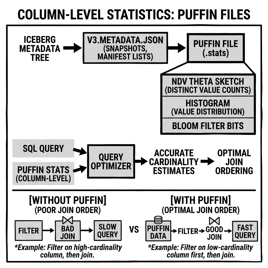
Storage Architecture: Puffin Files

Apache Iceberg introduced the Puffin file format as the container for table-level statistics. A Puffin file is an Iceberg-specific binary format with the following structure:

• A 4-byte magic header (P U F 1).
• A sequence of binary blobs, each containing one statistical artifact (a Theta Sketch, Bloom Filter, histogram, etc.) for a specific column and snapshot.
• A footer containing the metadata for all blobs: their type (identified by a canonical string like "apache-datasketches-theta-v1"), the column they describe, their byte offset within the file, and their size.
• A 4-byte magic footer marker.

Puffin files are referenced by name from the Iceberg Snapshot or from dedicated Statistics files referenced by the table metadata. The separation of statistics from the main metadata files (Manifest Files) allows statistics to be updated independently — you can re-compute NDV estimates without modifying the core table metadata, and you can expire old statistics without affecting the data or snapshot history.

Triggering Statistics Collection

Unlike file-level statistics (which are always computed at write time by the Parquet writer), table-level statistics in Puffin files require explicit computation through a separate operation. In most Iceberg-compatible engines, this is triggered by the ANALYZE TABLE command:

ANALYZE TABLE orders COMPUTE STATISTICS FOR ALL COLUMNS;

This command reads the table’s data, computes Theta Sketch NDV estimates for every column, generates histograms for configured columns, and writes the results to a new Puffin file. The operation can be compute-intensive for large tables, so it is typically scheduled as a periodic maintenance operation (daily, weekly, or after major data loads) rather than run after every write.

The query engine’s CBO module reads the Puffin statistics when it begins planning a query. If Puffin statistics are present and recent (i.e., the table has not changed dramatically since they were computed), the CBO produces accurate cardinality estimates. If statistics are absent or stale, the CBO falls back to default heuristics.

The Staleness Problem

Column-level statistics are a snapshot of the data at the time of collection. As new data is written and old data is deleted, the statistics become progressively staler and less accurate. A table that receives 10 million new rows per day will have NDV estimates from yesterday’s ANALYZE TABLE run that systematically undercount distinct values in columns populated by new data.

Staleness has direct consequences for CBO accuracy. If the optimizer uses a stale NDV estimate of 10 million distinct customers when the table actually has 15 million (after 30 days of growth since the last ANALYZE), it may underestimate the hash table size for a GROUP BY on customer_id, causing memory spills during the GROUP BY execution.

Strategies for managing statistics staleness:

Scheduled ANALYZE jobs: Run ANALYZE TABLE nightly or weekly during low-traffic windows. Accept that statistics are never perfectly current but are always within a defined staleness bound.

Incremental statistics collection: Compute statistics only for newly added data files (using Iceberg’s incremental statistics framework), and merge new Theta Sketches with existing ones using the sketch union operation. This avoids full-table reads on each statistics update.

Adaptive query execution: Some query engines (Spark with AQE enabled, Trino with dynamic filtering) can collect runtime statistics during query execution and adjust the query plan mid-execution based on observed actual cardinalities, partially compensating for stale pre-query statistics.

The Full Statistics Hierarchy in Query Execution

For a production lakehouse query, column-level statistics operate at multiple stages of the query execution lifecycle:

Stage 1 — Metadata Planning (Manifest-level file skipping): The query engine reads Iceberg Manifest Files and uses file-level lower_bounds/upper_bounds to eliminate data files before opening any Parquet file.

Stage 2 — Scan Planning (Row group skipping): For surviving data files, the query engine reads the Parquet footer and uses row-group-level min/max statistics to skip irrelevant row groups within the file.

Stage 3 — CBO Join Ordering (Before any execution): Before Stage 1 even begins, the query optimizer uses Puffin-stored NDV estimates and histograms to determine the optimal join order and strategy for the full query plan.

Stage 4 — Adaptive Re-planning (Mid-execution): Engines with Adaptive Query Execution can observe actual intermediate result cardinalities during execution (after Stage 2) and modify the remaining query plan to better match the actual data.

This four-stage process, each level informed by different categories of column-level statistics, is what separates a high-performance modern lakehouse from a naive Parquet-over-S3 data dump.

Conclusion

Column-Level Statistics are the invisible infrastructure that makes fast, cost-efficient lakehouse query execution possible. At the file and row group level, min/max bounds and null counts enable the IO reduction that transforms full-table scans into targeted reads of only the relevant data. At the table level, NDV estimates via Theta Sketches and value distribution histograms stored in Puffin files enable the cost-based optimization decisions that turn an O(N²) hash join into an O(N) broadcast join, a 10-minute aggregation into a 30-second one, and a 50GB memory allocation into a 500MB one. Engineers who invest in collecting, maintaining, and refreshing comprehensive column-level statistics — at both the file metadata level and the table statistics level — will consistently outperform teams that rely on raw data volume and compute brute force to compensate for query plans built on inaccurate cardinality guesses.

Visual Architecture