Compute Engine

In traditional data warehousing, storage and compute were inextricably linked. The database software that stored the data on disk was exactly the same software that executed SQL queries against it. You could not upgrade one without upgrading the other. If you needed more processing power to run complex end-of-month reports, you had to buy a larger database appliance, which also gave you more storage capacity whether you needed it or not.

The data lakehouse architecture fundamentally breaks this monolith through the separation of compute and storage. In a lakehouse, data is stored in open formats (like Parquet and Apache Iceberg) on commodity cloud object storage. The system that actually processes that data—the Compute Engine—is a completely separate layer.

A Compute Engine is a distributed software framework designed to read data from storage, execute transformations, aggregations, or analytical queries against that data across a cluster of machines, and return the results. Because it is decoupled from storage, you can scale the compute engine up during peak analytical hours and scale it down to zero overnight, paying only for the processing power you actually use. Even more importantly, because the storage uses open formats, you can point multiple different compute engines at the exact same data simultaneously.

How a Distributed Compute Engine Works

While different compute engines are optimized for different workloads, they share a similar distributed architecture.

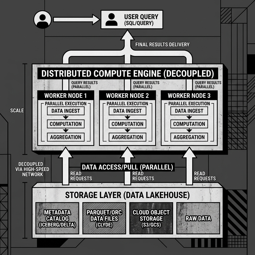
When a user or application submits a query (e.g., a SQL SELECT statement), it arrives at a Coordinator Node (sometimes called a Master or Leader node). The coordinator is the brain of the engine. It parses the SQL, checks the syntax, and consults the metadata catalog (like an Iceberg catalog) to determine exactly which data files in object storage contain the required records.

The coordinator then generates an execution plan. It breaks the massive query down into hundreds or thousands of smaller, parallel tasks. It then distributes these tasks across a cluster of Worker Nodes (or Executors).

The worker nodes do the heavy lifting. Each worker independently connects to the object storage layer, downloads its assigned data files into memory, and performs the required filtering, joining, and aggregation. If a worker node crashes mid-query, the coordinator detects the failure and simply reassigns that specific task to a surviving worker, ensuring fault tolerance. Finally, the workers send their partial results back to the coordinator, which assembles the final answer and returns it to the user.

Diagram 1: Compute Engine Architecture

Types of Compute Engines

Because compute is decoupled from storage in a lakehouse, organizations can choose specific compute engines optimized for specific types of workloads, all operating against the same underlying data.

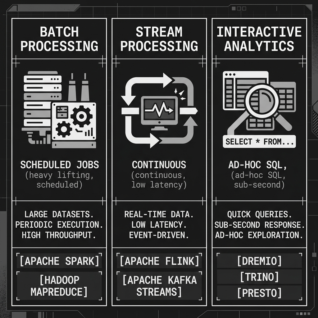
Batch Processing Engines are designed for heavy lifting. They excel at processing massive volumes of historical data, executing complex multi-stage ETL transformations, and training machine learning models. They prioritize fault tolerance and high throughput over sub-second latency. If a job takes four hours to process ten terabytes of data, that is acceptable, provided it completes reliably. Apache Spark is the undisputed industry standard for batch processing compute.

Stream Processing Engines are designed for continuous, low-latency execution. Rather than waking up on a schedule to process a massive batch of historical files, streaming engines run continuously, processing individual events or micro-batches the moment they arrive. They are used for real-time dashboarding, anomaly detection, and fraud alerting. Apache Flink and Spark Structured Streaming are the dominant engines in this category.

Interactive Analytics Engines (often called MPP SQL engines) are designed for speed. They prioritize sub-second query response times for human analysts and BI dashboards. They achieve this speed through sophisticated query optimization, advanced memory management (often using Apache Arrow for columnar in-memory processing), and aggressive caching of data and query plans. They are not designed for massive ETL jobs; they are designed to answer questions fast. Dremio and Trino (formerly PrestoSQL) are the leading interactive analytics compute engines.

Diagram 2: Compute Engine Workload Types

The Power of Engine Interoperability

The greatest advantage of the lakehouse architecture is that these different compute engines do not require different copies of the data.

In a modern data stack, an organization might use Apache Flink to stream raw clickstream data continuously into a Bronze Apache Iceberg table. Every night, an Apache Spark batch job wakes up, reads that Bronze table, performs complex deduplication and sessionization logic, and writes the results into a Silver Iceberg table. Simultaneously, hundreds of business analysts are using Dremio to execute sub-second interactive SQL queries against that exact same Silver table to populate their Tableau dashboards.

Three entirely different compute engines—one for streaming, one for batch, one for interactive analytics—are all operating against the exact same data lakehouse storage layer. The organization uses the optimal engine for each specific task without ever moving or copying the underlying data files. This engine interoperability is the defining technical achievement of the open data lakehouse.