Hilbert Curves

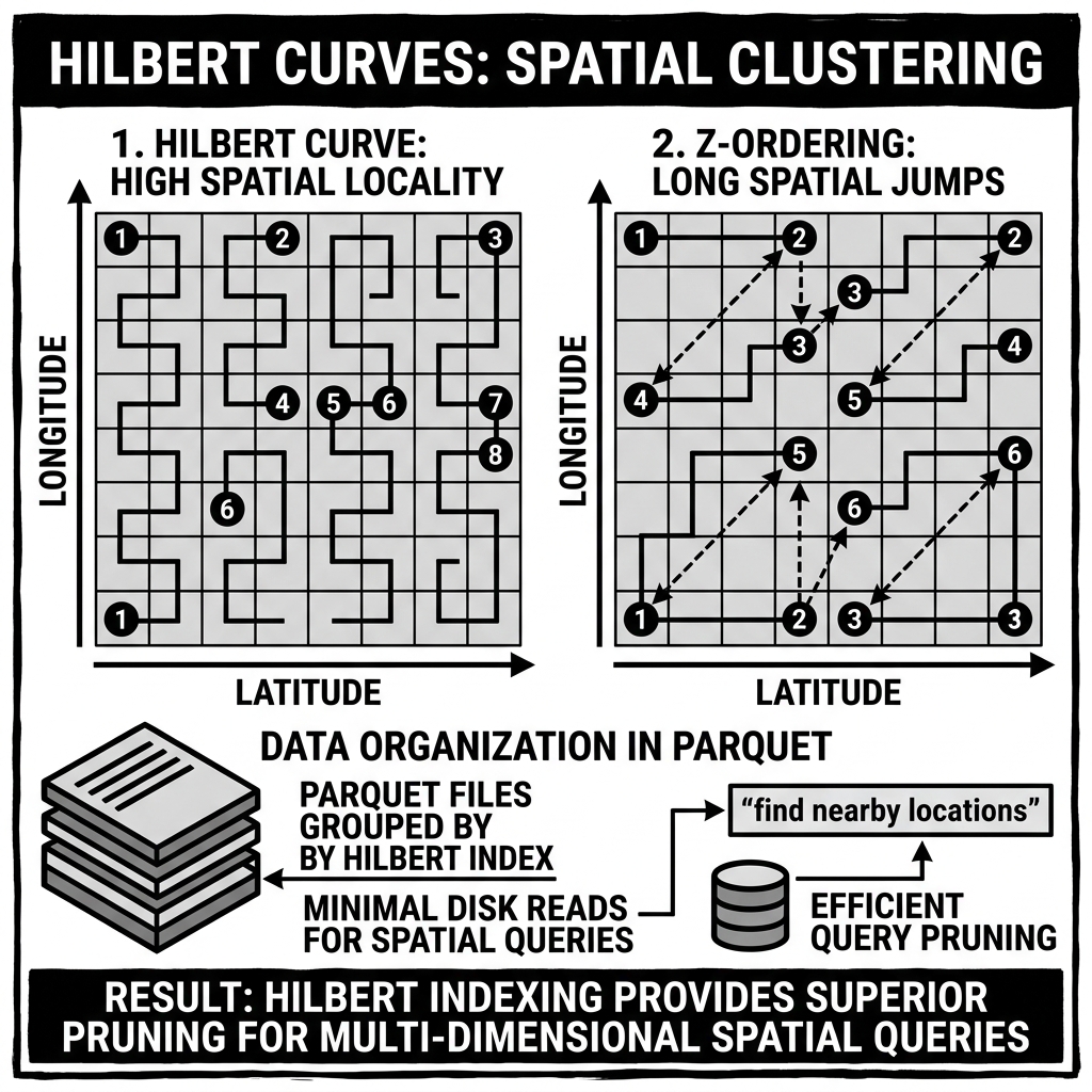
The Hilbert Curve is a mathematically elegant space-filling curve first described by mathematician David Hilbert in 1891. Like all space-filling curves, it traces a continuous path through a multi-dimensional space, visiting every point exactly once and reducing that multi-dimensional geometry to a single linear ordering. Unlike simpler space-filling curves such as the Z-curve (Morton curve), the Hilbert Curve is specifically constructed to minimize discontinuous “jumps” — abrupt transitions in the linear order where geometrically adjacent points in the original space are mapped far apart in the 1D linear index.

In the context of data engineering and data lakehouse architectures, the Hilbert Curve has emerged as the mathematically superior alternative to Z-Ordering for multi-dimensional data clustering. Its exceptional locality preservation properties make it the foundation for state-of-the-art clustering implementations, most notably Databricks’ Liquid Clustering feature, which uses Hilbert curve ordering as its core data layout algorithm.

To understand why the Hilbert Curve matters for data engineers, it is necessary to understand both the geometry of space-filling curves and the precise way that superior locality preservation translates into better query performance through data skipping.

The Geometry of Space-Filling Curves

A space-filling curve is a curve that, in its infinite limit, passes through every point of a bounded multi-dimensional space exactly once. For data engineering purposes, we are working with discrete approximations — finite-depth space-filling curves that divide the space into a finite number of cells and traverse them in a specific order.

The Construction of the Hilbert Curve

The Hilbert Curve is constructed through a recursive subdivision process. At each recursion level, the 2D unit square is divided into four quadrants. The curve visits each quadrant exactly once in an order that ensures adjacent quadrants in the path are also geographically adjacent in the space. The key construction rule is that at each subdivision, the curve’s entry and exit points for each sub-quadrant are chosen to maintain geographic adjacency with the neighboring sub-quadrants.

At recursion level 1, the Hilbert Curve visits four cells in a U-shape: bottom-left, top-left, top-right, bottom-right. At recursion level 2, each of those four cells is further divided into four sub-cells, and the Hilbert Curve within each sub-cell is oriented (rotated or reflected) to ensure that the curve’s exit from one sub-cell connects directly and adjacently to its entry into the next sub-cell.

The critical property that emerges from this recursive, adjacency-preserving construction: two points that are geographically near each other in the original 2D space almost always receive Hilbert curve indices that are near each other in the 1D linear order. The curve visits the entire geographic space in a sequence that strongly respects spatial neighborhoods.

The Z-Curve’s Locality Problem

To appreciate the Hilbert Curve’s advantage, compare it to the Z-curve (Morton curve), which was discussed in the Z-Ordering article.

The Z-curve is constructed by simple bit-interleaving: for 2D coordinates (X, Y), the Z-curve index is computed by interleaving the binary digits of X and Y. This is computationally trivial — just bit-shift and OR operations. However, the Z-curve has a well-known locality failure mode: large, discontinuous jumps between geometrically adjacent points at the boundaries between the “Z” shapes that give the curve its name.

Consider two points that are geographically adjacent but lie on opposite sides of a Z-curve boundary. Their X coordinates might be very similar (differing by 1 in the last bit), but their Z-curve indices may differ enormously — because that last differing bit, when interleaved with the Y coordinate bits, can shift the entire upper half of the index. These boundary jumps mean that cells that are geographically neighbors in the original space can be placed far apart in the Z-curve’s 1D ordering, undermining the spatial locality the curve is supposed to provide.

The Hilbert Curve is specifically engineered to eliminate these boundary jumps. By carefully controlling the orientation (rotation and reflection) of the curve at each recursive subdivision, the Hilbert construction ensures that the curve’s path never makes a large jump — every consecutive pair of cells in the 1D order is also a geographic neighbor in the 2D space. This is a much stronger locality guarantee than the Z-curve provides.

Quantifying the Locality Advantage

The mathematical measure of a space-filling curve’s locality is its clustering quality — specifically, the ratio of the average 1D distance between pairs of points to their average geometric distance in the original multi-dimensional space. A perfect locality-preserving ordering would have this ratio equal to 1.0 for all pairs of points. A random ordering would have a high ratio.

For 2D data, the Hilbert Curve achieves a clustering quality approximately 15–25% better than the Z-curve. This advantage grows significantly in higher dimensions (3D, 4D, 5D+), where the Z-curve’s boundary jumps become more frequent and more severe. In a 4-column clustering scenario (common in lakehouse workloads: user_id, region, product_category, date), the Hilbert Curve can achieve 30–40% better locality than the Z-curve.

The practical consequence for data skipping is direct: tighter locality means tighter per-file min/max statistics for all clustered columns, which means the query engine can skip more files for the same set of query predicates. A 30% improvement in locality translates to roughly a 20–30% additional reduction in bytes read for typical multi-predicate queries.

Hilbert Curves in Data Lakehouse Implementations

Delta Lake Liquid Clustering

Databricks’ Liquid Clustering feature, introduced in Delta Lake 3.1, uses Hilbert Curve ordering as its core data layout algorithm. When clustering columns are defined for a Delta table:

ALTER TABLE orders CLUSTER BY (customer_id, region);

Delta Lake computes the Hilbert curve index for each record based on its customer_id and region values, sorts the records by their Hilbert index, and writes them into new Parquet data files in Hilbert-sorted order. The result is that records with similar customer_id and region values are physically co-located in the same files, with per-file min/max statistics for both columns being tight and selective.

The key architectural improvement of Liquid Clustering over traditional Z-Order OPTIMIZE is that it applies the Hilbert clustering incrementally. New data files written by insert operations are clustered before being written. Existing un-clustered files are progressively re-clustered by background OPTIMIZE operations without requiring a full-table rewrite. This eliminates the expensive full-table OPTIMIZE operations that Z-Order ZORDER BY requires every time the table’s data changes substantially.

Apache Iceberg and the Sort Order Spec

Apache Iceberg’s architecture supports multi-column sort orders through the Sort Order Spec — a metadata structure that defines which columns the data files in the table are sorted by, and in what order. Iceberg’s rewriteDataFiles maintenance procedure can apply these sort orders to reorganize existing files.

While Iceberg’s core specification does not prescribe a specific space-filling curve for multi-column sort orders, query engines and catalog implementations can apply Hilbert or Z-Order sorting as their rewrite strategy. Dremio’s Iceberg table optimization, for example, applies Hilbert curve clustering when performing multi-column data reorganization, producing the same locality-preserving layout as Liquid Clustering but within the Iceberg metadata framework.

Computing the Hilbert Index: Technical Details

Computing a Hilbert curve index for a multi-dimensional record requires more computation than the Z-curve’s simple bit interleaving. The standard algorithm for Hilbert index computation uses a lookup table approach that, for each subdivision level, applies the appropriate rotation or reflection transformation to the current sub-square based on which quadrant the point falls in.

The steps for a 2D point (X, Y) with a target precision of N bits per dimension:

1. For each of N precision levels (from most significant to least significant bit):

   • Determine which quadrant of the current square the point falls in (00, 01, 10, or 11 based on the current-level bits of X and Y).
   • Append the quadrant index to the Hilbert code.
   • Apply the appropriate rotation/reflection transformation to the remaining sub-square coordinates based on which quadrant was entered.

2. The resulting N×2-bit string is the Hilbert index.

For practical implementations at 32-bit precision per dimension, the lookup table for the rotation/reflection state transitions is small (16 entries for 2D, 64 for 3D) and can be precomputed. Modern implementations compute Hilbert indices at throughputs of hundreds of millions of records per second per CPU core, making the computational overhead negligible compared to the IO cost of reading and writing the Parquet files being clustered.

When to Use Hilbert vs. Z-Order

Given that the Hilbert Curve provides superior locality, the question arises: is there ever a reason to use Z-Ordering instead?

Z-Ordering’s Remaining Advantages

Computational simplicity: Z-curve index computation is several times faster than Hilbert index computation due to the bit-interleaving approach versus the recursive state-machine approach. For systems processing extremely high volumes of records in real-time, this difference can matter. In batch clustering operations on data lakehouse files, however, the computation is so fast relative to the IO cost of reading and writing Parquet files that this advantage is practically irrelevant.

Legacy ecosystem compatibility: Z-Order ZORDER BY has been the standard in Delta Lake deployments for several years, with a large body of operational experience, documentation, and tooling. Teams with existing Z-ordered tables do not need to immediately migrate to Hilbert-based Liquid Clustering. Z-Ordering continues to provide substantial performance improvements over unoptimized layouts.

Simplicity of the index arithmetic: For educational purposes, explaining Z-Ordering requires only understanding bit interleaving, which most engineers can grasp immediately. The Hilbert Curve’s recursive rotation-and-reflection construction requires more mathematical background. For teams building custom clustering implementations without access to a mature Hilbert index library, Z-Ordering may be the more practical choice.

Hilbert Curve’s Clear Superiority

For production deployments on modern lakehouse platforms (Databricks Liquid Clustering, Dremio Hilbert-based optimization), the Hilbert Curve’s superiority is clear and should be the default choice:

• Better locality preservation means better data skipping, which means lower query latency and lower compute cost.
• The improvement is most pronounced for higher-cardinality columns and multi-column clustering scenarios — precisely the scenarios where Z-Ordering’s boundary jump problem is most severe.
• The incremental clustering architecture of Liquid Clustering (which uses Hilbert ordering) eliminates the full-table rewrite cost of traditional Z-Order OPTIMIZE, making operational maintenance far less expensive.

The Connection to Liquid Clustering’s Automatic Adaptability

One of the most important features of Liquid Clustering (beyond its use of Hilbert curves) is that the clustering is not fixed at table creation time. The clustering columns can be changed:

ALTER TABLE orders CLUSTER BY (product_id, order_date);

When the clustering definition changes, Delta Lake begins writing new files with the new clustering. Old files retain their original layout. Progressive background OPTIMIZE operations gradually re-cluster the old files under the new definition. At no point is the table locked or unavailable, and there is no expensive all-at-once rewrite.

This adaptability is architecturally impossible with traditional partitioning (which requires rewriting the entire table to change partition columns) and operationally complex with Z-Order OPTIMIZE (which requires re-running the full OPTIMIZE after any significant data change). Liquid Clustering’s combination of Hilbert curve locality and incremental application represents a qualitative improvement in both query performance and operational simplicity.

Conclusion

The Hilbert Curve is not merely a mathematical curiosity — it is the theoretically optimal space-filling curve for multi-dimensional data clustering in practical lakehouse data engineering contexts. Its recursive, adjacency-preserving construction eliminates the boundary jump problem that limits Z-curve (Morton code) locality, producing 15–40% better data clustering quality depending on the number of dimensions. This translates directly into tighter per-file column statistics, more effective query-time data skipping, and materially lower query latency for multi-predicate analytical workloads. Its adoption as the core algorithm in Databricks’ Liquid Clustering represents the state of the art in lakehouse data layout optimization, and understanding its properties is essential for any data engineer making informed decisions about clustering strategy, query performance optimization, and the choice between traditional partitioning, Z-Ordering, and modern Hilbert-based clustering.

Visual Architecture