Partition Pruning

Partition Pruning is the most powerful form of data skipping available to query engines in the data lakehouse. While other skipping mechanisms (min-max statistics, Bloom Filters, row-group pruning) operate at the file or sub-file level, partition pruning operates at the directory or logical table segment level — eliminating entire categories of files from the query plan before any file metadata is consulted. A single partition pruning decision can remove 364 out of 365 date partitions from a query’s scan scope, reducing the data read by 99.7% before any other optimization is applied.

The concept of data partitioning predates the modern data lakehouse by decades. Relational databases have supported table partitioning since the 1990s. The Apache Hive data warehouse, which formed the foundation of the first generation of open data lakes, adopted directory-based partitioning as its primary data organization mechanism. The modern Open Table Formats — Apache Iceberg and Delta Lake — have both preserved and significantly advanced the partition pruning concept, each with distinct architectural approaches that produce different capabilities and trade-offs.

The Fundamental Concept: Partitioning as Pre-Computed Data Segmentation

Partitioning is the practice of physically separating a table’s rows into distinct, non-overlapping segments based on the values of one or more designated partition columns. Each partition contains only the rows where the partition column equals a specific value (or falls within a specific range).

The direct consequence of this physical separation is that a query containing an equality predicate on the partition column (WHERE partition_col = value) can confine its scan to the single partition matching that value, completely ignoring all other partitions. The query engine does not read a single byte from any non-matching partition. This is not statistical skipping (which says “this file probably doesn’t contain matching rows”) — it is structural skipping (which says “this partition mathematically cannot contain matching rows, because all rows with different partition values are physically stored elsewhere”).

The Cardinality Constraint on Partition Key Selection

The critical operational constraint of partitioning is the relationship between partition key cardinality and operational viability:

Too few distinct values (low cardinality): Partitioning by a boolean column (is_active: two values) creates two partitions, each containing 50% of the table’s data. A query filtering WHERE is_active = true still reads 50% of the table — minimal improvement. The partition granularity is too coarse to provide meaningful skipping.

Too many distinct values (very high cardinality): Partitioning by user_id (millions of distinct values) creates millions of partitions. A table with 1 trillion rows and 10 million users creates 10 million partitions — each containing 100,000 rows on average. Each partition maps to a physical directory with potentially hundreds of small Parquet files (the dreaded “small file problem”). The metadata overhead for tracking millions of partitions becomes the performance bottleneck, not the data IO.

The optimal cardinality range: Partition columns should have enough distinct values to divide the data into meaningfully distinct segments (providing high selectivity), but not so many that the number of partitions becomes operationally unwieldy. Date columns (365 values per year) and month columns (12 values per year) are classic examples of well-chosen partition keys: they divide the data into regularly-sized segments that align naturally with common query patterns (queries almost always filter by date range), and their cardinality scales manageable.

Partition Implementations: Hive-Style vs. Iceberg Hidden Partitioning

The two major approaches to partition implementation in the lakehouse ecosystem have fundamentally different trade-off profiles.

Hive-Style Partitioning: The Legacy Approach

In the traditional Hive-style partitioning model (inherited by Delta Lake and most early data lake implementations), partition values are encoded directly in the file system directory structure using key=value naming:

s3://bucket/table/
  event_year=2026/
    event_month=05/
      event_day=18/
        file_001.parquet
        file_002.parquet
  event_year=2026/
    event_month=05/
      event_day=17/
        file_001.parquet

The partition columns (event_year, event_month, event_day) are typically stored as explicit columns in each Parquet file as well, despite also being encoded in the directory path. This redundancy exists because many query engines read the partition value from the directory path (faster, no need to open the file) rather than from the actual column data (requires decompressing and reading the column).

Advantages of Hive-style:

• Simple to understand and operate.
• Directly visible in object storage browsers — a human can navigate the partition hierarchy intuitively.
• Wide compatibility: any query engine that can list directories and parse key=value naming can infer partition structure without requiring a catalog.

Disadvantages of Hive-style:

• Redundant data: The partition column values are stored both in the directory path and in each file’s actual column data, wasting storage and requiring data writers to produce the partition directory structure correctly.
• Partition column exposure: Users must include partition columns in all INSERT statements and must know the partition scheme to write data correctly. Changing the partition scheme requires rewriting all existing data.
• Directory listing cost: On object storage (S3, GCS), listing the full partition directory tree is an expensive O(N) operation where N is the number of distinct partition values. For a table with 10,000 date partitions, the partition discovery operation requires hundreds or thousands of LIST API calls against the object storage service.
• Date format coupling: Queries must use the exact date format encoded in the directory path. Querying WHERE event_day = DATE'2026-05-18' might fail if the directory encodes it as event_day=20260518 (no hyphens), requiring format conversion.

Apache Iceberg Hidden Partitioning: The Modern Approach

Apache Iceberg introduced Hidden Partitioning as a fundamentally different approach that decouples the partition scheme from the user-facing table interface.

In Iceberg, partitioning is defined by a Partition Spec — a metadata structure that maps source column names to partition transforms. Transforms include:

• identity(col): Partition by the raw column value (similar to Hive-style).
• year(timestamp_col): Extract the year from a timestamp and partition by year.
• month(timestamp_col): Extract the year-month from a timestamp.
• day(timestamp_col): Extract the calendar date from a timestamp.
• hour(timestamp_col): Extract the year-month-day-hour from a timestamp.
• bucket(N, col): Hash the column value into one of N buckets.
• truncate(W, col): Truncate the column value to the first W characters (for strings) or to a multiple of W (for integers).

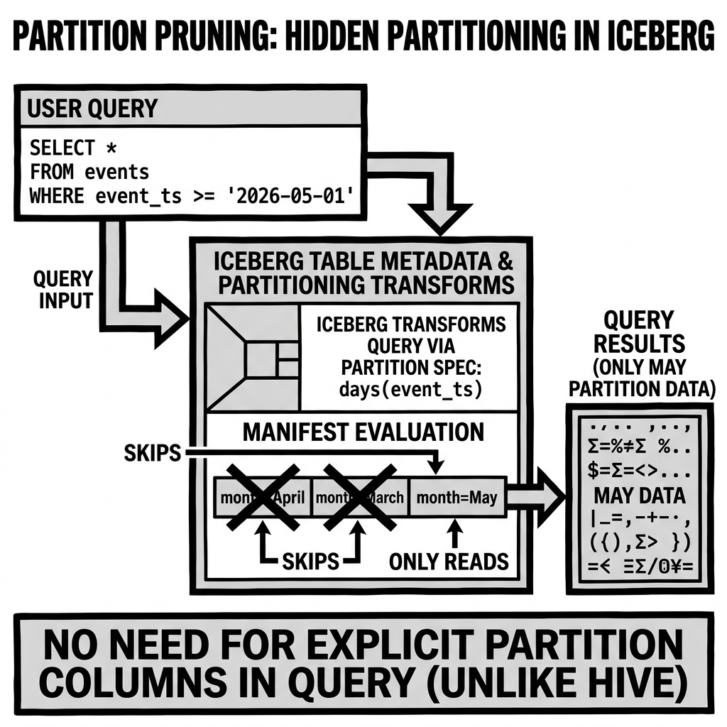
The critical property of Iceberg’s partition transforms is that they are invisible to the end user writing queries. A user does not need to know that the table is partitioned by month(event_timestamp). They simply write:

SELECT * FROM events WHERE event_timestamp BETWEEN '2026-05-01' AND '2026-05-31';

The Iceberg query planning layer automatically translates this predicate against the raw event_timestamp column into a partition filter against the computed month partition values, then prunes all month partitions outside the query’s date range. No user-side awareness of the partition scheme is required.

The Key Advantages of Hidden Partitioning:

• No partition columns in data: Parquet files don’t need to store redundant partition columns — the partition values are tracked in the Iceberg Manifest File metadata, not in the data files themselves. This eliminates redundant storage.
• No user-visible partition syntax: Users write queries against the natural column names. The partitioning is an implementation detail that the table format manages internally.
• No directory listing overhead: Partition pruning is performed by evaluating partition bounds in the Iceberg Manifest Files — a fast, metadata-only operation that doesn’t require any file system listing.
• Format-independent partition values: The partition value representation in the Manifest is format-independent. Whether the source column uses ISO-8601 timestamps or POSIX epoch integers, the Iceberg partition transform produces a canonical partition value that the query engine evaluates consistently.

Delta Lake’s Approach

Delta Lake uses Hive-style partitioning for its physical data layout (partition directories with key=value naming). However, Delta’s _delta_log stores partition values for each file in the add action’s partitionValues field, allowing partition pruning to be performed by reading the transaction log rather than by listing file system directories. This is faster than raw directory listing but still requires maintaining the physical directory structure.

Delta Lake’s OPTIMIZE command (especially with Liquid Clustering) is gradually moving toward a model where explicit partitioning is less necessary, replacing coarse directory partitioning with fine-grained Hilbert clustering that provides similar data skipping benefits without the operational constraints of managing partition directories.

Partition Pruning: The Execution Mechanics

Iceberg Partition Pruning Execution

1. Query planning begins: The query planner receives the parsed query and identifies predicates on columns (e.g., event_timestamp BETWEEN '2026-05-01' AND '2026-05-31').

2. Partition predicate translation: The planner evaluates which partition values could contain rows satisfying the predicate. For a month(event_timestamp) partition, the relevant partition values are those corresponding to months with any overlap with the date range: month 2026-05 (and potentially the edge months if the range crosses month boundaries).

3. Manifest List scan: The planner reads the Snapshot’s Manifest List. For each Manifest File, it evaluates the partition summary bounds (the min and max partition values across all files in the manifest) against the translated partition filter. Manifests with no matching partition values are skipped — their Manifest Files are not read.

4. Manifest File scan: For surviving Manifests, the planner reads each Manifest File and evaluates each file entry’s stored partition value against the partition filter. Files from non-matching partitions are excluded from the query plan.

5. File-level statistics evaluation: The remaining candidate files (those in matching partitions) are subject to file-level min-max statistics evaluation for additional pruning (as described in the File Skipping article).

The result: only files in the matching month partitions reach the file-level statistics evaluation stage. Files from all other months are completely eliminated in Step 4.

Delta Lake Partition Pruning Execution

1. The engine reads the Delta table’s transaction log (checkpoint + recent JSON commit files) to reconstruct the complete current set of active data files with their partitionValues.

2. The engine filters the active file set by evaluating each file’s partitionValues against the query’s partition predicates.

3. Files from non-matching partitions are excluded from the scan plan.

4. File-level statistics (stored in the stats field of the add action) are applied for further within-partition pruning.

The Partition Evolution Problem

A fundamental limitation of traditional Hive-style partitioning is that changing the partition scheme requires rewriting all existing data. If a table was originally partitioned by month(event_date) and you want to switch to day(event_date) (because data volume has grown and monthly partitions are now too coarse), you must re-read every existing file and re-write it to the new partition directory structure. For a petabyte-scale table, this is a multi-day, multi-million-dollar migration effort.

Iceberg’s Partition Evolution solves this by storing multiple Partition Spec versions in the table metadata. Each data file is tagged with the Partition Spec ID under which it was written. When a new Partition Spec is introduced:

• New data files are written under the new spec.
• Old data files remain under their original spec.
• Queries against the table correctly apply the appropriate partition filter for each file based on its spec ID.

A query filtering by event_date = '2026-05-18' on a table that has files from both a monthly spec and a daily spec will:

• For old files (monthly spec): filter by the month partition value derived from 2026-05-18 (month 2026-05).
• For new files (daily spec): filter by the day partition value derived from 2026-05-18 (day 2026-05-18).

No data rewriting required. The partition evolution is a pure metadata operation.

The Compaction Caveat

The one operational subtlety of partition evolution in Iceberg is the interaction with compaction. If a compaction job merges files from two different partition specs into a single output file, the resulting file doesn’t cleanly belong to either spec. The safe practice is to always compact within a single partition spec version — either by configuring compaction to preserve partition boundaries, or by running compaction only on the older files before the spec evolution takes effect.

Choosing the Right Partition Strategy

Scenario	Recommended Partition Strategy
Time-series data with primarily temporal queries	Partition by day(timestamp) or month(timestamp)
Large multi-region table with per-region analysis	Partition by region (if few regions) or bucket(N, region_id)
E-commerce orders with date + category queries	Partition by day(order_date), Z-Order by category
IoT sensor data with per-device queries	Partition by day(event_time), Bloom Filter on device_id
Event log data with no clear partition key	Partition by hour(ingest_time) (ingestion time is always available)
Table expected to grow from daily to monthly partitions	Use Iceberg hidden partitioning from the start to enable zero-cost evolution

Conclusion

Partition Pruning is the foundation of all lakehouse query performance at scale. Its ability to eliminate entire categories of files — not through probabilistic statistics but through the mathematical guarantee that non-matching partitions cannot contain matching rows — makes it the highest-leverage optimization available in the query planner’s toolkit. The evolution from Hive-style directory-based partitioning (simple but operationally rigid) to Iceberg’s hidden partitioning with logical transforms and metadata-driven partition bounds (more powerful, more flexible, operationally invisible to users) represents the single most impactful architectural improvement in how data lakehouse systems organize and access data. Every data engineer designing a lakehouse table schema should begin with the partition key selection — it is the architectural decision with the largest long-term impact on query performance, operational flexibility, and storage efficiency.

Visual Architecture