Z-Ordering

Z-Ordering is a multi-dimensional data clustering technique used in data lakehouse environments to physically co-locate records with similar values across multiple columns within the same data files, dramatically improving the effectiveness of file-level data skipping for multi-predicate analytical queries. It is one of the most impactful performance optimization strategies available to data engineers working with large Parquet-based tables in Apache Iceberg and Delta Lake environments.

To understand Z-Ordering, you must understand the problem it solves, the mathematics of the space-filling curve that makes multi-dimensional co-location possible, the practical mechanics of implementing it in a lakehouse pipeline, and the specific workload patterns where it delivers the most dramatic performance gains.

The Root Problem: The Curse of Dimensionality in File Skipping

Data skipping is the foundational mechanism that makes large-scale lakehouse queries fast. Every Parquet file stores per-column min/max statistics in its row group footer. Every Iceberg Manifest File stores per-column min/max statistics for each data file it tracks. When a query engine plans a query with a predicate (e.g., WHERE region = 'EU'), it reads these statistics and skips any file where the region column’s min value is greater than ‘EU’ or max value is less than ‘EU’ — the file cannot possibly contain any matching rows. This is pure statistical pruning, zero data bytes read.

Data skipping works beautifully when the table is sorted or partitioned by the predicate column. If you ORDER BY region, all EU rows cluster together in a small number of files, and all non-EU files are skipped instantly. The predicate-column statistics are tight and selective.

The Single-Column Sorting Problem

Sorting by a single column optimizes data skipping for queries filtering on that column, but creates a fundamental trade-off for all other columns. Consider a table sorted by event_date. Queries filtering by event_date will have extremely tight statistics and skip aggressively. But queries filtering by user_id will be hopeless — users with the same user_id are scattered randomly across every date partition, so every file potentially contains rows for any given user_id. The user_id min/max statistics across files will be nearly as wide as the full range of user IDs in the entire dataset, providing essentially zero skipping value.

Real analytical workloads rarely filter by exactly one column. A typical dashboard query might filter by country, product_category, AND date_range. A typical machine learning feature pipeline might filter by user_segment AND event_type. A compliance query might filter by account_status AND transaction_type AND reporting_period.

Linear single-column sorting — the standard tool for data layout optimization — can only optimize for one of these predicate columns at a time. The others remain unoptimized, forcing full scans through many files that should logically be skippable.

This is the core problem that Z-Ordering solves.

The Mathematics: Morton Space-Filling Curves

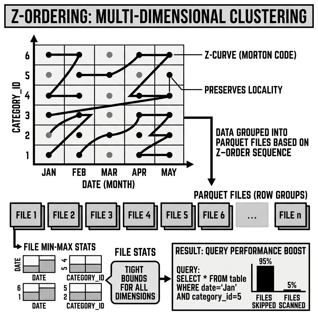
Z-Ordering is named after the Z-curve, also called the Morton curve after its inventor G. M. Morton, who described it in 1966 in a paper about geographic data organization. The Z-curve is a specific type of space-filling curve — a mathematical construct that traces a continuous path through a multi-dimensional space, visiting every point exactly once.

The Bit-Interleaving Construction

The key insight of the Z-curve is that it maps multi-dimensional coordinates to a single linear index using bit interleaving. Given two integers X and Y representing 2D coordinates, their Z-curve index (called the Morton code) is computed by interleaving the binary representations of X and Y:

If X = 5 = 101 in binary, and Y = 3 = 011 in binary, then:

X bits:  1   0   1
Y bits:    0   1   1
Interleaved: 10 01 11 = Morton code

The resulting single integer encodes both the X and Y coordinates simultaneously. Crucially, points that are geographically close in the 2D space (similar X and Y values) tend to have similar Morton codes — meaning they cluster together in the 1D sorted order.

For three or more dimensions, the same bit-interleaving principle applies: the bits from all dimensions are interleaved in round-robin fashion. For a 4-column Z-Order on columns A, B, C, D, the Morton code is produced by taking the most significant bit of A, then the most significant bit of B, then C, then D, then the second-most significant bit of A, and so on.

Locality Preservation

The critical property of the Morton code that makes it useful for data clustering is locality preservation: records with similar values across all Z-ordered columns will have similar Morton codes, and therefore will appear near each other in the sorted order. This is not perfect — there are boundary artifacts in the Z-curve where two points that are geometrically close but on different “arms” of the Z-curve end up with very different Morton codes. But statistically, across large datasets, the locality preservation is strong enough to dramatically tighten per-file column statistics compared to either random file ordering or single-column sorting.

Applying Z-Ordering in Practice

Delta Lake: OPTIMIZE ZORDER BY

In Delta Lake, Z-Ordering is applied through the OPTIMIZE command with the ZORDER BY clause:

OPTIMIZE orders ZORDER BY (customer_id, region, product_category);

This command triggers a full rewrite of the table’s data files. The compute engine:

1. Reads all existing Parquet files in the table (or in the specified partition range).
2. Computes the Morton code for each record based on the Z-ordered column values.
3. Sorts all records by their Morton code.
4. Writes the records in Morton code order into new, larger Parquet files (typically targeting 128MB–256MB file sizes).
5. Records the old files as remove actions and the new files as add actions in a new Delta commit.

After the operation, records with similar values across customer_id, region, and product_category are co-located in the same or adjacent Parquet files. The per-column min/max statistics in each file are now tight across all three columns simultaneously, not just one.

Apache Iceberg: Sorting and Clustering

Iceberg does not provide a native ZORDER BY SQL command equivalent to Delta’s, but it supports multi-column sort orders through its Sort Order Spec and the rewriteDataFiles maintenance procedure. The SORT strategy in rewriteDataFiles can sort by multiple columns, achieving linear multi-column sorting. For true Z-Order clustering in Iceberg, some execution engines provide their own Z-Order implementations as a rewrite strategy.

Dremio’s Iceberg support, for example, provides Z-Order clustering as a table maintenance operation, applying Morton code sorting to Iceberg data files using the same mathematical approach as Delta’s ZORDER BY. Spark with the Iceberg connector can also apply Z-Order sorting through the SparkActions.rewriteDataFiles().option("sort-order", ...) API.

The Cardinality Requirement

Z-Ordering is most effective on columns with high cardinality — many distinct values distributed across the full value range. The statistical pruning improvement from Z-Ordering depends on the per-file min/max statistics becoming significantly tighter than they would be in a random file layout. This tightening only occurs if there are enough distinct values to create meaningful clustering.

Z-Ordering on a boolean column (is_active: only two distinct values, true and false) provides minimal benefit — half the records are true and half are false, so almost every file will contain both values, and the min/max statistics will span the full [false, true] range in almost every file regardless of the clustering. Z-Ordering on a user_id column with 10 million distinct values provides enormous benefit — the Morton code will cluster user IDs with similar values together, and each file will cover a narrow range of user IDs with tight min/max statistics.

The Diminishing Returns of Multiple Columns

While Z-Ordering can technically sort by any number of columns, its effectiveness diminishes as more columns are added. The fundamental reason is geometric: in higher-dimensional spaces, the locality preservation of the Z-curve degrades because the boundary artifacts (where nearby points in high-dimensional space have very different Morton codes) become more frequent.

The practical rule of thumb, borne out by production experience across many lakehouse deployments, is that Z-Ordering beyond 3–4 columns provides diminishing returns and is often not worth the additional compute cost of the rewrite. Engineers should select the 2–4 columns most commonly used together in query predicates for their analytical workloads.

The Workloads Where Z-Ordering Delivers Maximum Impact

Multi-Predicate Ad Hoc Analytical Queries

Business intelligence tools and data science notebooks that generate ad hoc SQL queries with multiple predicate columns are the primary beneficiary of Z-Ordering. A query like:

SELECT sum(revenue) 
FROM orders 
WHERE country = 'US' 
  AND product_line = 'Electronics' 
  AND order_date BETWEEN '2026-01-01' AND '2026-03-31'

On a Z-Ordered table (ZORDER BY country, product_line, order_date), the query engine can skip the vast majority of files because each file’s min/max statistics for all three columns are tight. The US Electronics orders from Q1 2026 are physically clustered together in a handful of files. The engine reads only those files.

On an unoptimized table (random file layout), every file potentially contains some US orders, some Electronics orders, and some Q1 2026 orders — but no individual file is likely to contain all three predicates simultaneously. The engine cannot skip any file confidently, and must scan the entire table.

Production case studies from Databricks and other lakehouse operators consistently report 50–95% reductions in bytes read and query latency improvements of 3–10x for multi-predicate queries on well-Z-Ordered tables.

CDC (Change Data Capture) Pattern Lookups

In a table that receives continuous CDC updates keyed on entity_id, analytical queries that need to find the current state of specific entities (WHERE entity_id = 12345) benefit enormously from Z-Ordering on entity_id. Rather than scanning every file to find the record for entity 12345 (which could be in any file given the temporal insertion order of CDC updates), the Z-Ordered layout clusters entities with similar IDs together, allowing the engine to identify and read only the few files that contain the target entity’s records.

Z-Ordering vs. Partitioning: When to Use Each

Z-Ordering and partitioning solve related but distinct problems.

Partitioning is appropriate for columns with low-to-medium cardinality and a clear, natural hierarchy that divides the data into non-overlapping segments. Partitioning by date means all data from 2026-05-18 is physically segregated from all other dates. The query engine can completely skip entire partition directories for date-filtered queries — it never reads a single byte from date=2026-05-17 when the query only needs date=2026-05-18. This is the strongest possible form of data skipping.

Z-Ordering is appropriate for columns with high cardinality where partitioning would create too many partitions (billions of distinct user_id values cannot be individually partitioned), or for secondary predicate columns where the primary partition already handles the highest-selectivity filter.

A common production pattern is to combine both: partition by date (low cardinality, deterministic data layout) and Z-Order by user_id and event_type (high cardinality secondary filters) within each date partition. The partition handles the coarse-grained data segmentation; the Z-Order handles fine-grained clustering within each partition.

Liquid Clustering: The Next Evolution

Delta Lake 3.1 introduced Liquid Clustering as the recommended successor to both traditional partitioning and Z-Ordering for new tables. Liquid Clustering uses Z-Order-style multi-dimensional co-location but applies it incrementally and adaptively rather than requiring a full-table rewrite every time the clustering is updated.

In Liquid Clustering, new data files are written with clustering applied immediately (without requiring a separate OPTIMIZE command), and existing files are progressively re-clustered by background OPTIMIZE operations. The clustering columns can be changed without a full-table rewrite. The system automatically adapts the clustering granularity based on data volume.

Liquid Clustering represents the same core idea as Z-Ordering — multi-dimensional locality for data skipping — implemented with significantly less operational overhead and more adaptability to changing query patterns.

Conclusion

Z-Ordering is one of the most powerful and practically impactful query optimization techniques available to data lakehouse engineers. By applying Morton space-filling curve sorting to reorganize Parquet data files so that records with similar values across multiple predicate columns are physically co-located, Z-Ordering tightens the per-file min/max statistics that query engines use for data skipping. For multi-predicate analytical workloads on large tables where no single partition column adequately concentrates the selectivity of typical queries, Z-Ordering consistently delivers 3–10x query latency improvements with storage costs comparable to simple file compaction. Understanding its mathematical foundation, its cardinality requirements, its diminishing returns beyond 3–4 columns, and its relationship to traditional partitioning is essential for any data engineer responsible for query performance optimization in a production lakehouse environment.

Visual Architecture